Post Stastics
- This post has 3767 words.
- Estimated read time is 17.94 minute(s).
Once a novice developer learns the basic syntax of their programming language, and begins writing anything more than simple hello-world type apps, they start to encounter problems. At first, these problems seem daunting. To find answers, they usually start hitting the various software development forums and social sites where their kindred spirits tend to congregate and start asking questions. Often these questions take the form of “How do I do XYZ? or “My program is very slow, how do I improve its performance?”
These novice developers often view the more experienced developers as some kind of oracles since they seem to have magical answers to their queries. But in truth, the more experienced developers simply have more knowledge gained from experience. They have been where you are now (if you’re in this position), and have learned that most of the magic incantations are grouped into something known as “Algorithms”. Most people have heard that an algorithm is simply a set of ordered steps used to produce a particular result. But most boot-camp grads and self-taught developers, simply don’t get introduced to algorithms and data structures well enough. They are typically more concerned with learning the language(s) and frameworks they intend to use, and then they want to start creating apps right away.
I’m not putting this down, by the way, I am a self-taught developer myself. I struggled for a few years before I got introduced to a set of recipes and patterns that eased my development experience. If you want to be a good developer, you’ll want to learn the basic algorithms for things like sorting, searching, and tree and graph traversal. You’ll also want to learn about algorithmic complexity in both space and time. Having this knowledge alone won’t make you a great developer, but you can’t be a rock star without it!
It is impossible to impart all you need to know in a single blog post, or even several blog posts. So I recommend you find yourself a couple of good books on the subject. I also recommend, watching some of the video lectures from EdX, OCW, Corusera, CS50, and Youtube videos.
What I would like to do here is give you a very brief and basic introduction to some of the classic algorithms using the Dart language. So let’s get started!
Algorithms and Data Structures
Algorithms and data structures go hand in hand. A data structure is basically the package you box your data up in. An algorithm is an ordered set of steps you apply to your data structure(s) to produce a desired outcome. Whether that be sorting your data, searching it for a particular value, or some other desired operation. Algorithms are applied to data and data structures package that data in some fashion.
Simple Data Structures
The simplest of all data structures is a simple memory location such as that used to store a byte value. This data structure can be thought of as a simple box with a byte value placed inside. However, this simple data structure is very important to developers who develop software for memory restricted systems such as embedded systems.
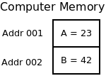
Discrete Cell Data Structure
Let’s say you are writing software for something like an AtTiny Microcontroller and you need to conserve as much memory as possible. You have two, byte values (A, B) and you need to swap their locations. However, you can’t afford to use another byte as temporary storage. How would you swap the bytes without using a third memory location?
At first, you may think this is impossible. If you write byte A into the location for value B, you’ll overwrite value B and won’t be able to place value B into the location for value A unless you first save value B somewhere. So how can we solve this issue? We can solve our dilemma with a little mathematics. Below is a simple algorithm to swap two values without using temporary storage for the intermediate value.
Given: A = 23, B = 42
Step 1. A = A + B  ->  65 = 23 + 42
Step 2. B = A - B  ->  23 = 65 - 42
Step 3. A = A - B  ->  42 = 65 - 23
Now, you may think this is the only way to achieve this swap. But the truth is there are many ways to complete the swap. A less obvious solution but one, more accustomed to embedded developers is to use the XOR (Exclusive Or) logic function. This algorithm is shown below:
Given: A = 23, B = 42
Step 1: A = A xor B  ->  61 = 23 xor 42
Step 2: B = A xor B  ->  23 = 61 xor 42
Step 3: A = A xor B  ->  42 = 61 xor 23
Now you may think that both of these solutions are equivalent. But you would be wrong! In the world of small microcontrollers, logic operations on byte values are quite common. Microcontrollers are often optimized for doing logical operations. Often the arithmetic operations such as adding and subtracting are slower and their opcodes require more room in ROM (program memory) than logic operations do. So it is often better to use the XOR solution.
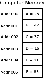
Linear Table -Data Structure
The linear table is usually referred to as a one dimensional array. This data structure is a simple linear list of adjacent memory cells. It is used to store a sequence of elements.
There are many algorithms that work upon arrays. Arrays are often used as adjacency lists, a data structure we will get to in a bit. They are quite powerful but also have a few drawbacks.
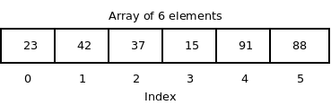
Let’s say you have an unordered array of six values (elements), and you want to find the largest value in the array. What steps would you take to locate the largest element?
Most people will do a simple linear search like that shown below:
Given: arr = [23, 42, 37, 15, 91, 88], index = 0, largest = 0

Step 1: While index is smaller than the length of the array arr:
step 2:    if arr[index] > largest then largest = arr[index]
step 3:    index = index + 1
step 4:    go to step 1
The above algorithm walks over every value in the array and saves the largest value seen so far in largest. It then increments the value of the index and examines the next location in the array, again saving the value from the array in largest if it is larger than the current value saved in largest. These steps repeat until every value in the array has been examined. This works pretty well and after all, you have to examine each element at least once to ensure you have the largest element in largest.
Now lets try another approach. This time we will walk up the array and compare adjacent values. If the value on the left (lowest index) is larger than the value on the right, we will swap the position of the values. In this way the largest value will bubble up to the end of the array.
Below is a sequence diagram of the steps needed to walk the largest value in the array to the end of the array.
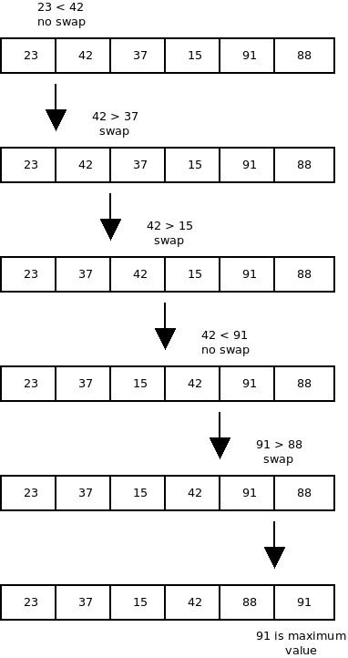
OK, so we’ve been showing sudo code and pretty pictures for a bit. Now its time to see some Dart code!
int maxValue(List<int> arr) {
  var index = 0;

  while (index < arr.length - 1) {
    if (arr[index] > arr[index + 1]) {
      var temp = arr[index + 1];
      arr[index + 1] = arr[index];
      arr[index] = temp;
    }
    index = index + 1;
  }
  // return last element of arr
  print('Arr: $arr');
  return arr[index];
}

void main() {
  var arr = [23, 42, 37, 15, 91, 88];
  var largest = maxValue(arr);
  print('The largest value is $largest');
}
Now it should be said here that I am not using the Dart language to its full potential here. My aim here is not to teach you Dart but to introduce you to some simple algorithms. So I have avoided using the features of the language that would complicate or obscure how the algorithm works. Instead, I am writing the most verbose code possible here.
If you enter and run the code above, you will see the output below:
Arr: [23, 37, 15, 42, 88, 91]
The largest value is 91
If you compare this result to the sequence diagram above you’ll see that the swaps were made every time the left value was larger than the right value. While here I used a temporary variable (temp) to store the value of arr[index]. I could have replaced the loop code with one of the swap methods used above. That way, the temp variable would not be needed.
So what is the advantage of using this method other than saving on a variable’s worth of memory? Well, here there really is none. So why did we go to all this trouble then? The reason for implementing the array swap here is so you can see this in action in a simple application. Next, we’re going to build upon this technique to implement a sorting algorithm.
Bubble Sort
Bubble Sort is an old sorting algorithm. It is sometimes referred to by other names such as Sinking Sort, Sifting Sort, and others. The algorithm is simple and so makes a good example for teaching sorting and searching algorithms in general. But it performs poorly in most cases. Bubble Sort does have one redeeming quality however, it is efficient at detecting whether a list is already sorted, and is often used in computer graphics to detect and correct small errors in almost-sorted arrays in linear time.
This occurs when two adjacent elements in the array have been placed in the wrong order. Then bubble sort can efficiently swap them back to the correct order. This is very handy for polygon sorting or Z-depth sorting where the position of a few polygons or sprites has changed their location in the Z-axis. I.e. moved closer or further away from the viewer. Bubble Sort also finds use in some polygon filling algorithms.
Bubble Sort however, is not generally efficient and it’s efficiency drops dramatically on lists of more than a few elements. So why teach it? Well, because it does have some use in detecting if a list is sorted, and it is one of the easiest to understand and comprehend sorting algorithms. So it makes a good introduction. I would recommend however, that unless you are only needing to test that a list is sorted or not, that you never use bubble sort in production code!
Alright, enough talk about its inefficiencies. How does it work? Well, bubble sort works just like our algorithm to find the largest value in the six-element array above. The only difference is, you need to run it over the array many times. Let’s revisit the largest value example above, only, this time let’s run the `maxValue` function twice and see the result.
int maxValue(List<int> arr) {
  var index = 0;

  while (index < arr.length - 1) {
    if (arr[index] > arr[index + 1]) {
      var temp = arr[index + 1];
      arr[index + 1] = arr[index];
      arr[index] = temp;
    }
    index = index + 1;
  }
  // return last element of arr
  print('Arr: $arr');
  return arr[index];
}

void main() {
  var arr = [23, 42, 37, 15, 91, 88];
  var largest = maxValue(arr);
  print('The largest value is $largest');
  largest = maxValue(arr);
  print('The largest value is $largest');
}
And the output is:
Arr: [23, 37, 15, 42, 88, 91]
The largest value is 91
Arr: [23, 15, 37, 42, 88, 91]
The largest value is 91
Notice here that the order of the values 15 and 37 have been swapped. With each run of the ‘maxValue’ function on the array, the array has additional elements sorted in the correct order. So how do we know how many times to run the 'maxValue‘ function? Generally, we will need to run the function length(arr) – 1 times. If the array has six elements we will generally need to run it five times. So the time complexity of bubble sort is O(n^2). This is very bad. Imagine if you had a list of ten million items to sort!
So lets see this complete algorithm in action with a loop to ensure the list gets fully sorted.
List<int> sortOnce(List<int> arr) {
  var index = 0;

  while (index < arr.length - 1) {
    if (arr[index] > arr[index + 1]) {
      var temp = arr[index + 1];
      arr[index + 1] = arr[index];
      arr[index] = temp;
    }
    index = index + 1;
  }
  return arr;
}

void main() {
  var arr = [23, 42, 37, 15, 91, 88];
  var sorted = [];

  print('Unsorted: $arr');
  for (var i = 0; i < arr.length-1; i++) {
    sorted = sortOnce(arr);
    print('Sort $i: $sorted');
  }
}
And the output:
Unsorted: [23, 42, 37, 15, 91, 88]
Sort 0: [23, 37, 15, 42, 88, 91]
Sort 1: [23, 15, 37, 42, 88, 91]
Sort 2: [15, 23, 37, 42, 88, 91]
Sort 3: [15, 23, 37, 42, 88, 91]
Sort 4: [15, 23, 37, 42, 88, 91]
The astute observers among you may realize that our list was sorted by the time we completed our third sorting. Yet, we still walked over our list two more times. This is a waste of time and a good indication that we can do better. A quick and simple optimization to bubble sort is to keep track of when we swap items. The first time we walk the list and do not swap an item, the list is fully sorted and we can stop. Let’s see this optimization in action:
void bubbleSort(List<int> arr) {
  var didSwap = false;

  print('Unsorted: $arr');

  for (var i = 0; i < arr.length - 1; i++) {
    didSwap = false;
    for (var j = 0; j < arr.length - 1; j++) {
      if (arr[j] > arr[j + 1]) {
        didSwap = true;
        var temp = arr[j];
        arr[j] = arr[j + 1];
        arr[j + 1] = temp;
      }
    }

    print('Sort $i: $arr');
    if (!didSwap) break;
  }
}

void main() {
  var arr = [23, 42, 37, 15, 91, 88];
  bubbleSort(arr);
}
OK, here we made several changes to the code to move all the logic into the ‘bubbleSort’ method. I replaced the ‘while’ loop with a ‘for’ loop and added a boolean value to flag when a swap takes place. If we went through the inner loop without swapping any values, we break out of the loops, ending the algorithm. If you run this code you’ll get the following output:
Unsorted: [23, 42, 37, 15, 91, 88]
Sort 0: [23, 37, 15, 42, 88, 91]
Sort 1: [23, 15, 37, 42, 88, 91]
Sort 2: [15, 23, 37, 42, 88, 91]
Sort 3: [15, 23, 37, 42, 88, 91]
Now, this isn’t a big difference in run time. We only saved an iteration. However, to see this optimization do more, add the following values to the array ‘arr’ in the main function.
var arr = [23, 42, 37, 15, 91, 88, 102, 100, 101];
If you run the code now you’ll get the following result:
Unsorted: [23, 42, 37, 15, 91, 88, 102, 100, 101]
Sort 0: [23, 37, 15, 42, 88, 91, 100, 101, 102]
Sort 1: [23, 15, 37, 42, 88, 91, 100, 101, 102]
Sort 2: [15, 23, 37, 42, 88, 91, 100, 101, 102]
Sort 3: [15, 23, 37, 42, 88, 91, 100, 101, 102]
As you can see, we sorted the list in the same four steps needed for the list of six integers. This is because we are able to place more than one value in its relatively correct position in a single pass. While our small optimization has helped us improve bubble sort, bubble sort is still far from being an optimal sorting algorithm.
Selection Sort
The Selection Sort algorithm splits an array into two parts. The sorted and the unsorted parts. It then repeatedly finds the smallest element (ascending order) in the unsorted part of the array and places it at the end of the sorted array. A diagram will help codify the idea:
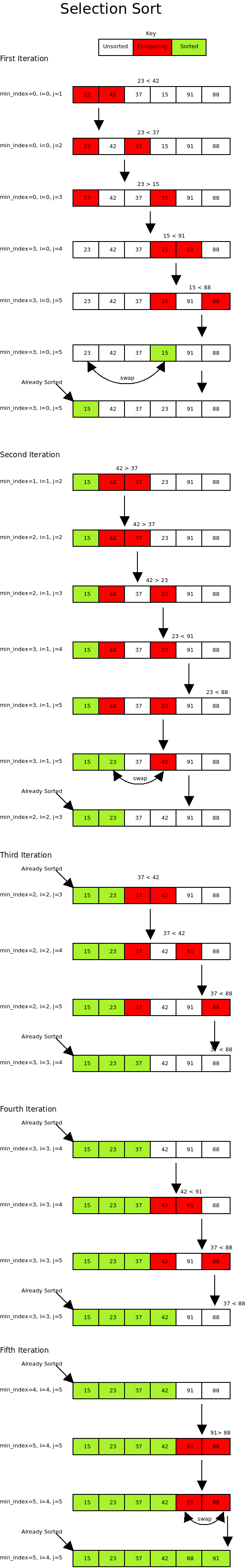
That took a lot of real estate to depict. But if you scroll through the diagram you’ll get the idea. Variable min_index always points to the smallest value left in the unsorted portion of the array. J is then used to walk over the remaining portion of the unsorted list, updating min_index as needed.
Alright, let’s see some code!
void selectionSort(List<int> arr) {
  var i = 0, j = 1;

  print('Unsorted: $arr');

  // Traverse through all array elements
  for (i = 0; i < arr.length; i++) {

    // Find the minimum element in remaining unsorted array
    var min_index = i;
    for (j = i + 1; j < arr.length; j++) {
      if (arr[min_index] > arr[j]) min_index = j; // Save minimum element's index
    }

    // Swap the found minimum element with the first element
    var temp = arr[min_index];
    arr[min_index] = arr[i];
    arr[i] = temp;

    print('Iter $i, arr: $arr');
  }

  print('Sorted: $arr');
}

void main() {
  var arr = [23, 42, 37, 15, 91, 88];
  selectionSort(arr);
}
If you run this code you’ll get the following output:
Unsorted: [23, 42, 37, 15, 91, 88]
Iter 0, arr: [15, 42, 37, 23, 91, 88]
Iter 1, arr: [15, 23, 37, 42, 91, 88]
Iter 2, arr: [15, 23, 37, 42, 91, 88]
Iter 3, arr: [15, 23, 37, 42, 91, 88]
Iter 4, arr: [15, 23, 37, 42, 88, 91]
Iter 5, arr: [15, 23, 37, 42, 88, 91]
Sorted: [15, 23, 37, 42, 88, 91]
OK, we’ve seen a few simple algorithms.We’ve seen bubble sort and selection sort and I have commented that bubble sort has poor performance in most cases. But how do you know how well an algorithm will perform and how can you compare algorithm performance? That will be our next topic!
Asymptotic Complexity and Analysis
Algorithms require time and memory space to run. When comparing two algorithms, you compare their runtimes and the memory space they use. However, we do not compare exact numbers, as this will depend greatly on the machine the algorithm is running on. For example, running a binary search on a 1990’s model HP Pavillion Desktop will provide much longer run times for the same size input when run on a modern mainframe such as the Z Series. Instead, we calculate how the runtime and memory space relates to the size of the input as the size of the input tends toward infinity. In other words, we only worry about very large inputs. When we are done we will end up with the Order of growth in runtime or memory size related to the growth in the input size. So what we record is the relationship between the size of the input and the rate of change in runtime or memory space used.
There are three performance vectors we are concerned about when we classify the performance of an algorithm. These are:
- O – (Big-Oh): The upper bound or maximum
- Ω – (Big Omega): The lower bound or minimum
- ϴ – (Theta): The average case
Entire books have been written on algorithmic complexity and asymptotic analysis so I wont be doing it justice here. I only want to wet your appetite so you’ll go explore additional materials on the subject.
You will hear many things about asymptotic complexity. Some good and some bad. An algorithm that works well in practice in the finite amount of space available and with finite inputs, doesn’t need to have good asymptotic complexity (good performance on a finite number of instances doesn’t imply anything regarding the asymptotic complexity). Similarly, an algorithm with good asymptotic complexity may not work well in practice over the range of inputs that we may be interested in (e.g. because of large constants). So, why do we use asymptotic complexity?
The truth is, we don’t have a better solution! The only other method is testing/benchmarking. We can program the algorithms, let them run on (a representative sample of) the finite input set, and compare the results. While this may seem a reasonable replacement, there are some problems with this approach:
- The results are not general in terms of machines. Run your benchmark on another computer and you get different results for sure, quantitatively, and perhaps even qualitatively.
- The results are not general in terms of implementation details. You literally compare programs, not algorithms. Small changes in the implementation can cause huge differences in performance.
- The results are not general in terms of programming languages. Different languages may cause very different results.
- In practice, input sets change and usually become larger over time. If you don’t want to repeat your benchmark every six months, your results will soon become worthless.
- If the worst-case is rare, a random input sample may not contain a bad instance. That is fair if you are concerned with average-case performance, but some environments require worst-case guarantees (real-time processing).
That said, ignoring all kinds of effects and constants in the analysis is typical. It serves to compare algorithmic ideas more than to pinpoint the performance of a given implementation. It is well known that this is a coarse measure and that a closer look is often necessary. For example, Quicksort is less efficient than Insertion sort for very small inputs. However, a more precise analysis is usually hard to complete.
Another, justification for the formal, abstract viewpoint is that on this level, things are often clearer. Thus, decades of theoretic study have produced a host of algorithmic ideas and data structures that are of use in everyday practice. The theoretically optimal algorithm is not always the one you want to use in practice – there are often other considerations besides performance to make. Asymptotic analysis provides us the best intuition for, and analysis of algorithms. It has become the standard method for and has proved sufficient in the general case for predicting performance.
Algorithm Analysis
As stated above we have three typical vectors we may use to define the performance of our algorithms. Big-Oh, Theta, and Big-Omega. Often we may only care about the worst possible runtime or the maximum amount of memory our algorithm will use. Sometimes, however, we may need to know the minimum time an algorithm will run. Most often, however, we will want to know the average running time or memory the algorithm will require. So how do we calculate this?
The asymptotic complexity can be computed as a count of all elementary operations. More easily, a count of all operations modifying data, or as a count of all comparisons. We then throw out all lower-order terms e.g. constants. Recall it is not the exact number of operations we are interested in. It is the growth in relationship to the input size that matters. So lower-order terms can be neglected. After all, if your algorithm takes 2 million steps another 3, 4, or even 1000 additional steps isn’t going to make much difference.
Below we have the function n f(n) with n as the input size. Each row contains a different input size. The remainder of each row shows the time required to process the given input for the given algorithmic complexity. Each column represents a progressively more complex algorithm.
| n f(n) | log n | n | n log n | n2 | 2n | n! |
|---|---|---|---|---|---|---|
| 10 | 0.003ns | 0.01ns | 0.033ns | 0.1ns | 1ns | 3.65ms |
| 20 | 0.004ns | 0.02ns | 0.086ns | 0.4ns | 1ms | 77years |
| 30 | 0.005ns | 0.03ns | 0.147ns | 0.9ns | 1sec | 8.4×10¹⁵yrs |
| 40 | 0.005ns | 0.04ns | 0.213ns | 1.6ns | 18.3min | — |
| 50 | 0.006ns | 0.05ns | 0.282ns | 2.5ns | 13days | — |
| 100 | 0.07 | 0.1ns | 0.644ns | 0.10ns | 4×10¹³yrs | — |
| 1,000 | 0.010ns | 1.00ns | 9.966ns | 1ms | — | — |
| 10,000 | 0.013ns | 10ns | 130ns | 100ms | — | — |
| 100,000 | 0.017ns | 0.10ms | 1.67ms | 10sec | — | — |
| 1,000,000 | 0.020ns | 1ms | 19.93ms | 16.7min | — | — |
| 10,000,000 | 0.023ns | 0.01sec | 0.23ms | 1.16days | — | — |
| 100,000,000 | 0.027ns | 0.10sec | 2.66sec | 115.7days | — | — |
| 1,000,000,000 | 0.030ns | 1sec | 29.90sec | 31.7 years | — | — |
While I’ve discussed a few points here on asymptotic complexity, I’ll recommend the codescope site: https://www.codesdope.com/course/algorithms-introduction/ and the bigocheatsheet site: https://www.bigocheatsheet.com/ for a better understanding.
As you can see, complexity really matters. I have seen programs that went from taking hours to run to only a few milliseconds by rewriting the algorithms used.
Conclusion
We’ve only touched the tip of the iceberg here. I may write more on algorithmic complexity in another post. For this series however, I simply want to show you some common algorithms and implement them in Dart. We will continue next time with more searching and sorting algorithms.
Until then, happy coding!