Post Stastics
- This post has 1537 words.
- Estimated read time is 7.32 minute(s).
Introduction
Control systems engineering stands as a cornerstone in modern technology, enabling the precision and stability of processes in diverse domains. Within this realm, the Proportional, Proportional-Derivative (PD), and Proportional-Integral-Derivative (PID) control algorithms play pivotal roles. This extensive guide navigates the intricate landscape of these control strategies, offering both theoretical insights and practical implementations in the C programming language. Through an immersive journey, we will uncover the evolution from basic Proportional control to the sophisticated PID control, all while presenting a plethora of code examples that illuminate the step-by-step construction of these algorithms.
The Essence of Proportional (P) Control
The Foundation of Proportional Control
Proportional (P) control serves as the bedrock upon which more advanced control algorithms are built. It operates by adjusting the control output in proportion to the current error, which is the difference between the desired setpoint and the actual process variable.
Mathematical Expression of P Control
Mathematically, the P control algorithm is expressed as:
[ u(t) = K_p \cdot e(t) ]
Where:
- (u(t)) is the control output at time (t)
- (K_p) is the proportional gain, determining the strength of the control action
- (e(t)) is the error signal at time (t), calculated as (e(t) = \text{setpoint} – \text{process variable})
Implementing P Control in C
Let’s embark on our journey by implementing the basic P control algorithm in the C programming language. Consider a scenario where we regulate the intensity of a light bulb to maintain a desired level of brightness.
Step 1: Initialization
Commence by initializing the essential variables:
#include <stdio.h>

// Constants
double setpoint_brightness = 80.0; // Desired brightness level
double current_brightness = 60.0; // Current brightness level

// Gain
double K_p = 0.8; // Proportional gain

// Control output
double control_output = 0.0;
Step 2: P Algorithm Implementation
Next, proceed with the P algorithm’s implementation:
double calculate_p_control() {
    // Calculate error
    double error = setpoint_brightness - current_brightness;

    // Calculate control output using P algorithm
    control_output = K_p * error;

    return control_output;
}
Step 3: Simulating P Control
Simulate the control process to observe how the P controller adjusts the control output to maintain the desired brightness level:
int main() {
    int time_step = 1; // Time step in seconds
    int simulation_time = 60; // Total simulation time in seconds

    for (int t = 0; t < simulation_time; t += time_step) {
        // Simulate brightness change (due to external factors)
        current_brightness += 1.0; // Increase by 1 unit per second

        // Calculate control output using P algorithm
        double p_output = calculate_p_control();

        // Apply control output to the system (light bulb, in this case)
        // For simplicity, we'll just print the control output
        printf("Time: %d seconds | P Control Output: %.2f\n", t, p_output);
    }

    return 0;
}
Unveiling the Proportional-Derivative (PD) Control Algorithm
Advancing Beyond P Control with PD Control
The Proportional-Derivative (PD) control algorithm refines the Proportional (P) control strategy by introducing the concept of rate of change. P control, while effective in reducing steady-state errors, can lead to oscillations around the desired setpoint. The PD control aims to mitigate this oscillation by incorporating the derivative of the error, enabling a more anticipatory response to changes.
The Mathematics Behind PD Control
Mathematically, the PD control algorithm computes the control output ((u(t))) as follows:
[ u(t) = K_p \cdot e(t) + K_d \cdot \frac{de(t)}{dt} ]
Where:
- (K_p) represents the proportional gain, influencing the control action based on the current error (e(t)).
- (K_d) is the derivative gain, emphasizing the control action based on the rate of change of the error ((de(t)/dt)).
The derivative term introduces stability by damping oscillations and expediting convergence to the setpoint. However, PD control may still struggle with addressing steady-state errors, necessitating further refinement.
Implementing PD Control in C
Building upon our foundational understanding, let’s proceed to implement the PD control algorithm in the C programming language. Our example scenario involves controlling the speed of a hypothetical vehicle. The goal is to maintain a target speed by adjusting the throttle.
Step 1: Initialization
Begin by initializing the essential variables:
#include <stdio.h>

// Constants
double setpoint_speed = 60.0; // Target speed in mph
double current_speed = 40.0; // Current speed in mph

// Gains
double K_p = 1.0; // Proportional gain
double K_d = 0.5; // Derivative gain

// Previous error for derivative calculation
double prev_error = 0.0;

// Control output
double control_output = 0.0;
Step 2: PD Algorithm Implementation
Proceed with the implementation of the PD algorithm:
double calculate_pd_control() {
    // Calculate error
    double error = setpoint_speed - current_speed;

    // Calculate rate of change of error
    double error_derivative = error - prev_error;

    // Calculate control output
    control_output = K_p * error + K_d * error_derivative;

    // Store current error for the next iteration
    prev_error = error;

    return control_output;
}
Step 3: Simulating PD Control
Now, simulate the control process to observe how the PD controller adjusts the control output to maintain the desired speed:
int main() {
    int time_step = 1; // Time step in seconds
    int simulation_time = 120; // Total simulation time in seconds

    for (int t = 0; t < simulation_time; t += time_step) {
        // Simulate speed change (due to incline, wind resistance, etc.)
        current_speed += 2.0; // Increase by 2 mph per second

        // Calculate control output using PD algorithm
        double pd_output = calculate_pd_control();

        // Apply control output to the system (throttle, in this case)
        // For simplicity, we'll just print the control output
        printf("Time: %d seconds | PD Control Output: %.2f\n", t, pd_output);
    }

    return 0;
}
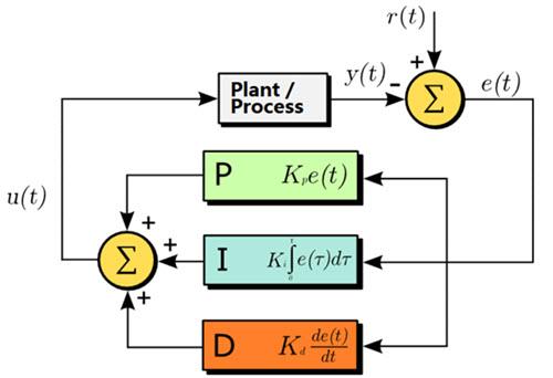
The Symphony of Proportional-Integral-Derivative (PID) Control
Achieving Harmony with PID Control
The Proportional-Integral-Derivative (PID) control algorithm amplifies the principles of PD control by introducing an integral component. The Integral (I) action addresses the challenge of persistent steady-state errors encountered by P and PD controllers. By considering the historical accumulation of error, the PID controller gains the power to eliminate long-term deviations from the set-point.
The Mathematics Behind PID Control
The PID control algorithm combines proportional, integral, and derivative terms to compute the control output ((u(t))) as follows:
[ u(t) = K_p \cdot e(t) + K_i \cdot \int_{0}^{t} e(\tau) d\tau + K_d \cdot \frac{de(t)}{dt} ]
Where:
- (K_p) is the proportional gain
- (K_i) is the integral gain
- (K_d) is the derivative gain
- (e(t)) is the error signal at time (t)
- (de(t)/dt) is the rate of change of the error
Implementing PID Control in C
Advancing further, let’s implement the PID control algorithm in the C programming language. Imagine a scenario where you are tasked with regulating the temperature of a furnace.
Step 1: Initialization
Start by initializing the essential variables:
#include <stdio.h>

// Constants
double setpoint_temperature = 200.0; // Desired temperature in Celsius
double current_temperature = 150.0; // Current temperature in Celsius

// Gains
double K_p = 1.5; // Proportional gain
double K_i = 0.2; // Integral gain
double K_d = 0.8; // Derivative gain

// Previous error and integral for calculations
double prev_error = 0.0;
double integral = 0.0;

// Control output
double control_output = 0.0;
Step 2: PID Algorithm Implementation
Proceed with the implementation of the PID algorithm:
double calculate_pid_control() {
    // Calculate error
    double error = setpoint_temperature - current_temperature;

    // Calculate integral term
    integral += error;

    // Calculate derivative term
    double error_derivative = error - prev_error;

    // Calculate control output
    control_output = K_p * error + K_i * integral + K_d * error_derivative;

    // Store current error for the next iteration
    prev_error = error;

    return control_output;
}
Step 3: Simulating PID Control
Simulate the control process to observe how the PID controller adjusts the control output to maintain the desired temperature:
int main() {
    int time_step = 1; // Time step in seconds
    int simulation_time = 180; // Total simulation time in seconds

    for (int t = 0; t < simulation_time; t += time_step) {
        // Simulate temperature change (heating/cooling process)
        current_temperature += 0.5; // Increase by 0.5 degrees Celsius per second

        // Calculate control output using PID algorithm
        double pid_output = calculate_pid_control();

        // Apply control output to the system (furnace, in this case)
        // For simplicity, we'll just print the control output
        printf("Time: %d seconds | PID Control Output: %.2f\n", t, pid_output);
    }

    return 0;
}
Strengths and Shortcomings
PID control is renowned for its versatility, combining the strengths of proportional, derivative, and integral actions. It provides a rapid response to changes, precise setpoint tracking, and robust performance in the presence of disturbances. However, tuning PID parameters can be intricate, and the integral term may lead to integral windup, especially in systems with saturation limits.
Applicability and Progression
PID control is apt for a wide range of systems, making it a mainstay in control engineering. Its adaptability suits processes with varying dynamics and disturbances. However, the behavior of the system should guide the choice of control strategy. If integral windup becomes problematic or faster settling times are imperative, advanced control strategies like model-based control or adaptive control should be considered.
Conclusion
Traversing the complex terrain of control systems, our journey from basic Proportional control to advanced PID control unveils an array of solutions tailored to diverse challenges. Each algorithm boasts distinctive strengths and weaknesses, aligning them with specific scenarios. Proportional control establishes stability, PD control mitigates oscillations, and PID control combines the trifecta of proportional, derivative, and integral actions for precise control.
As engineers, our choice of control algorithm stems from careful analysis of system behavior, dynamics, and constraints. With each step forward, we refine our ability to master control and guide systems toward desired outcomes. Through this guide, you’ve gained the tools to navigate the realm of control algorithms and orchestrate the symphony of control in diverse engineering domains.